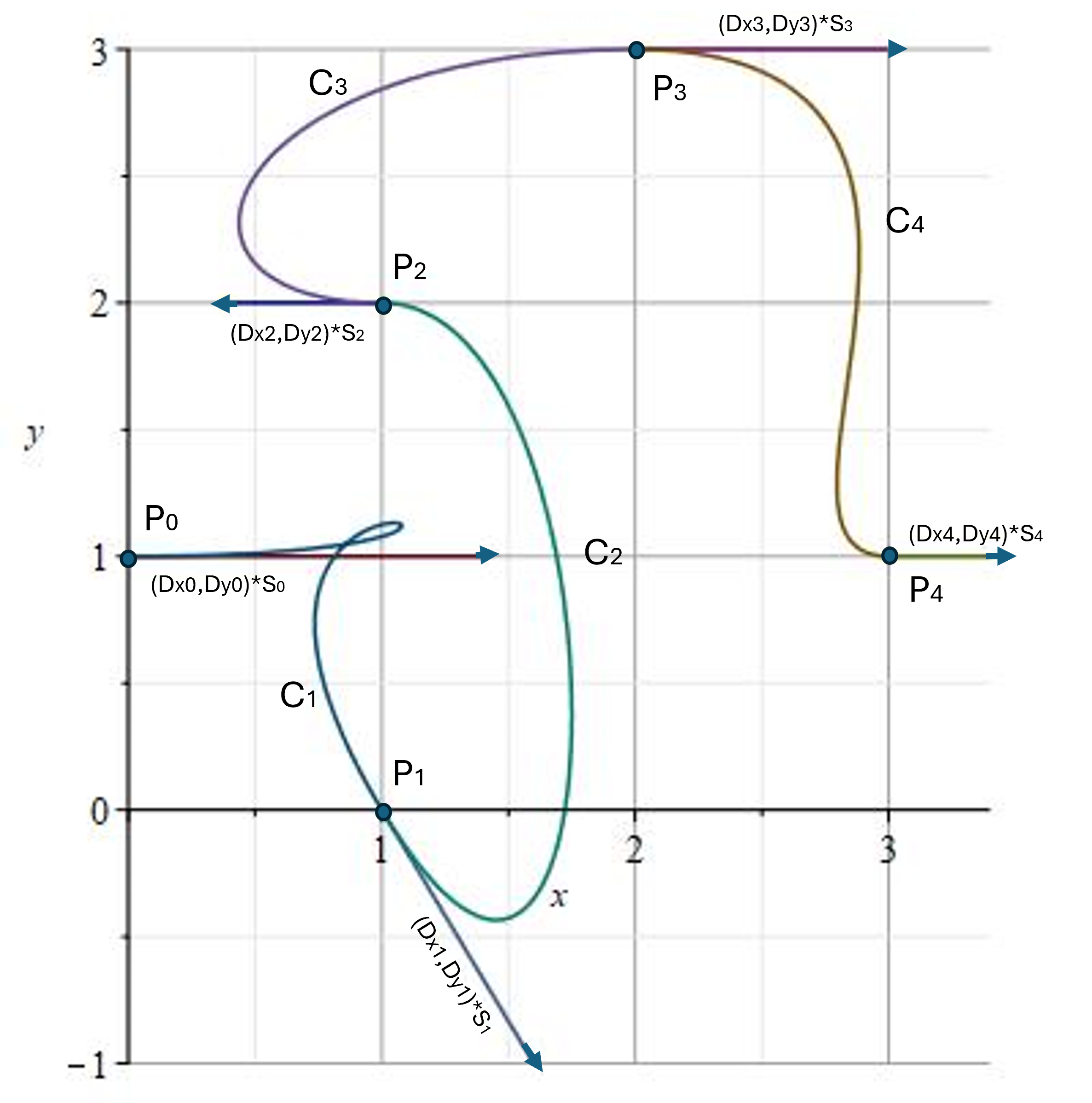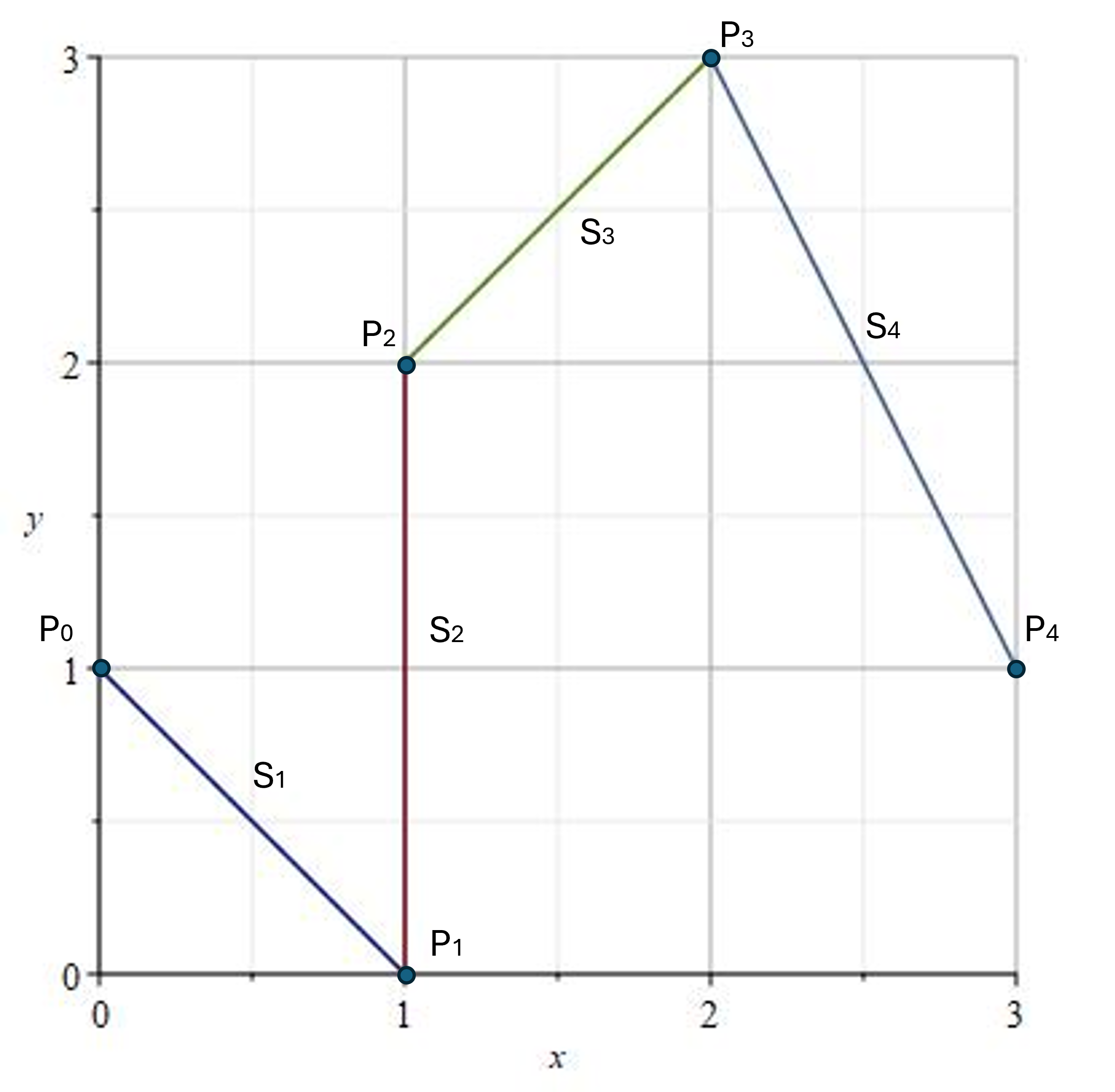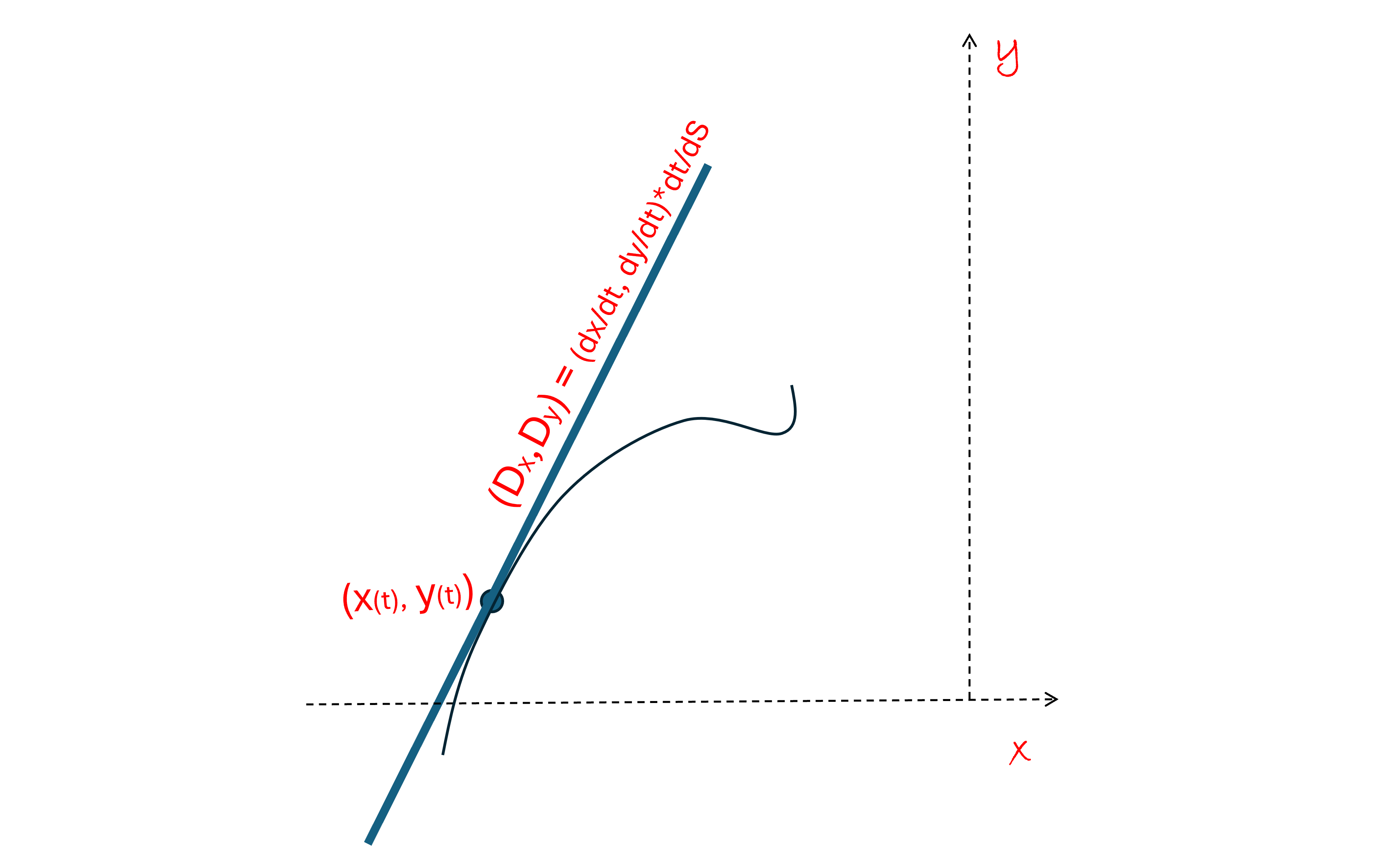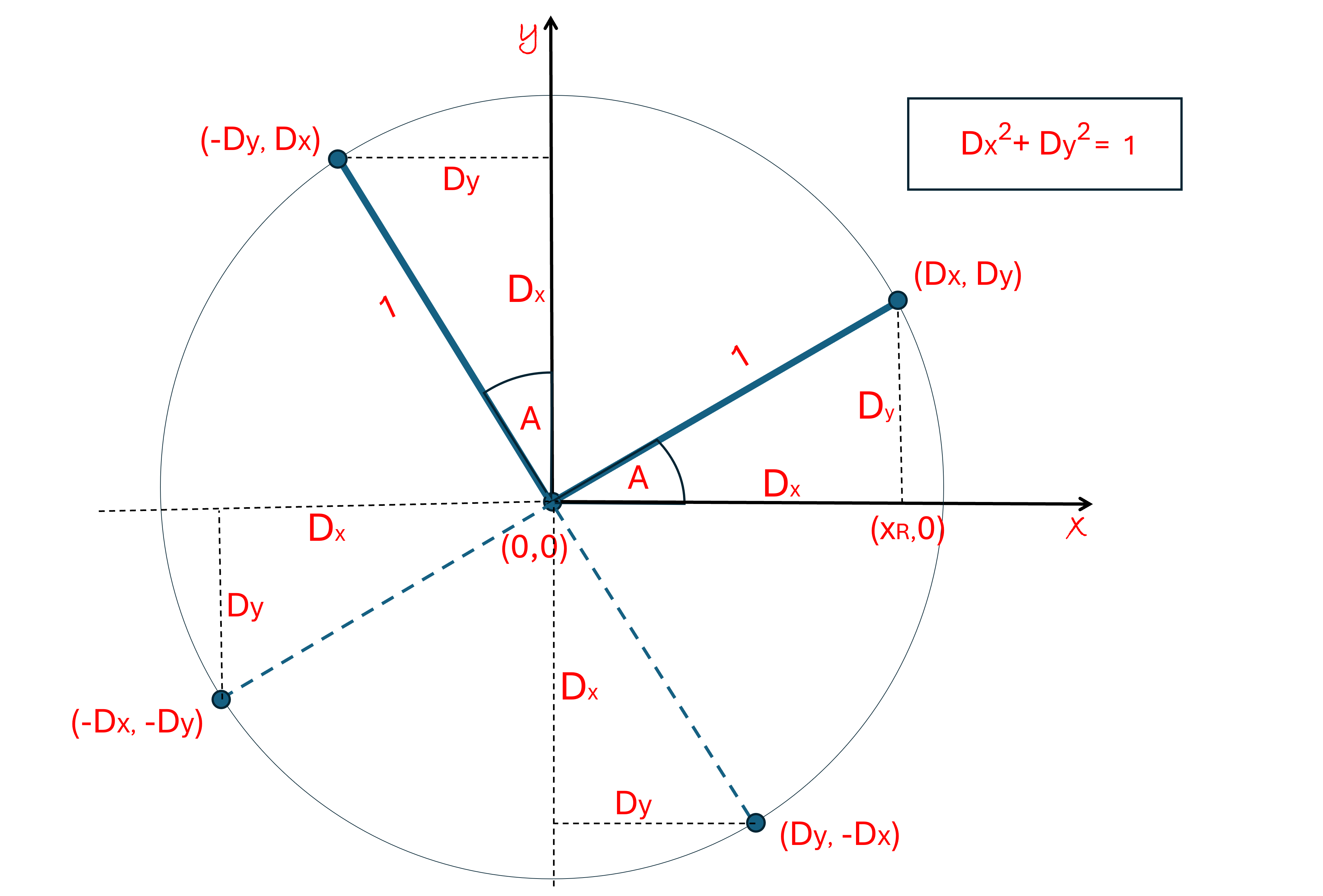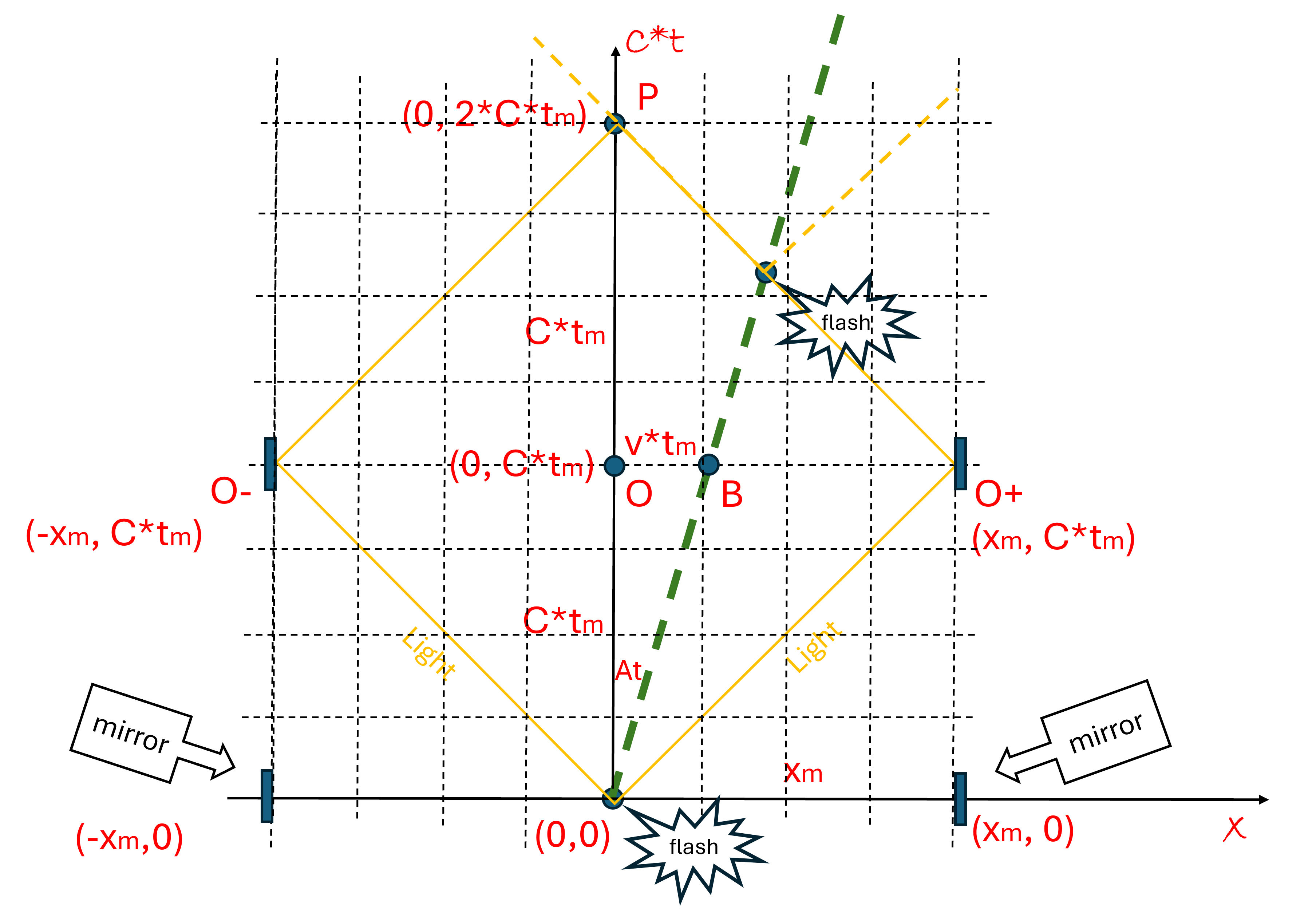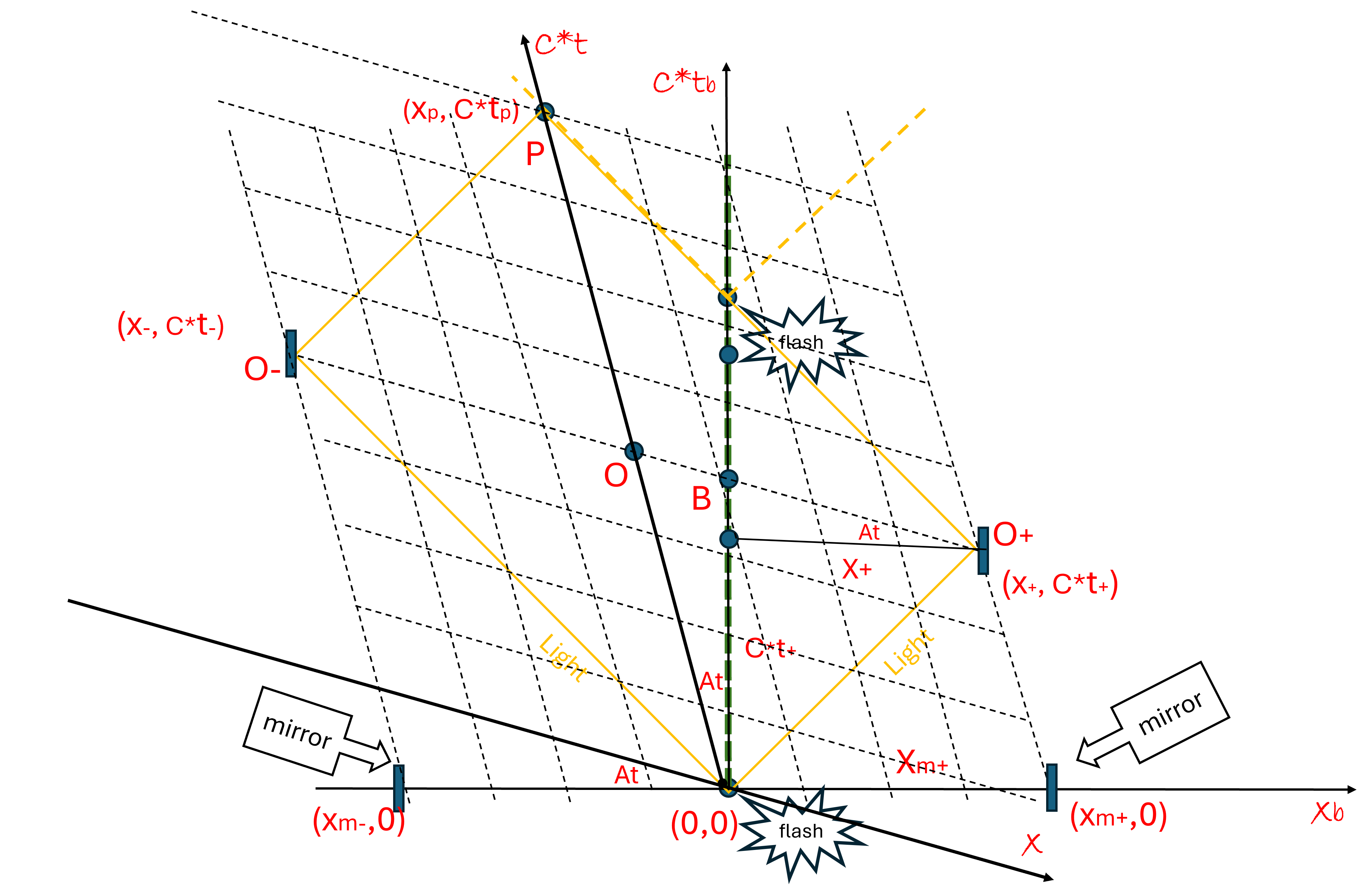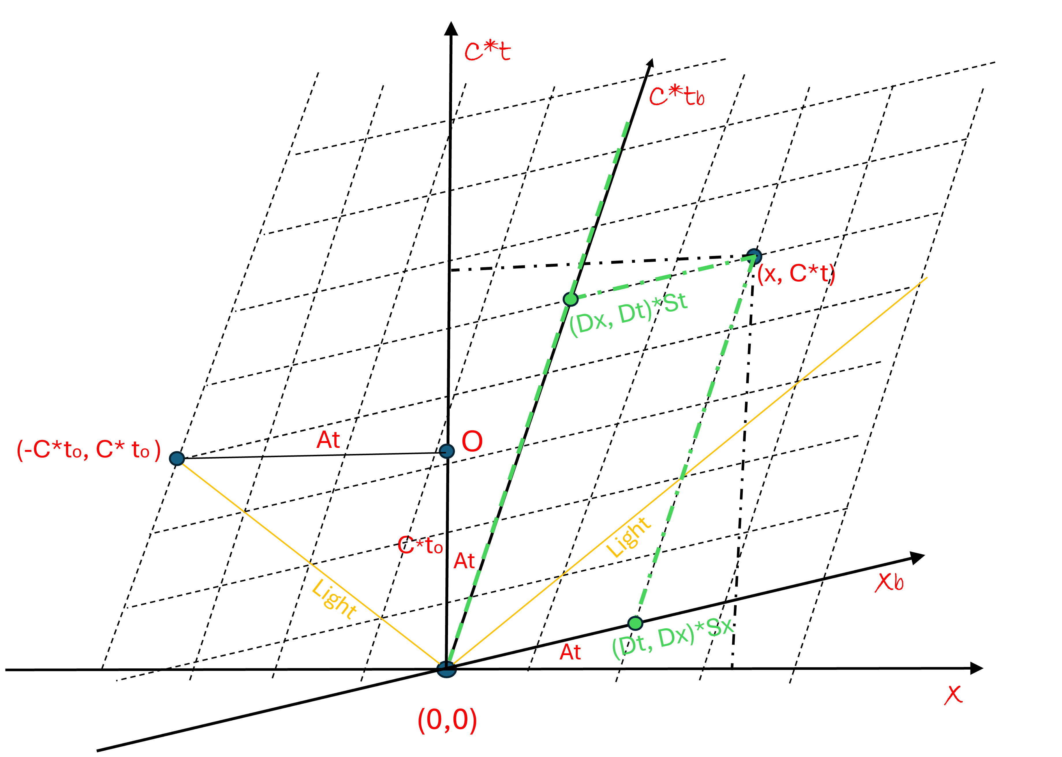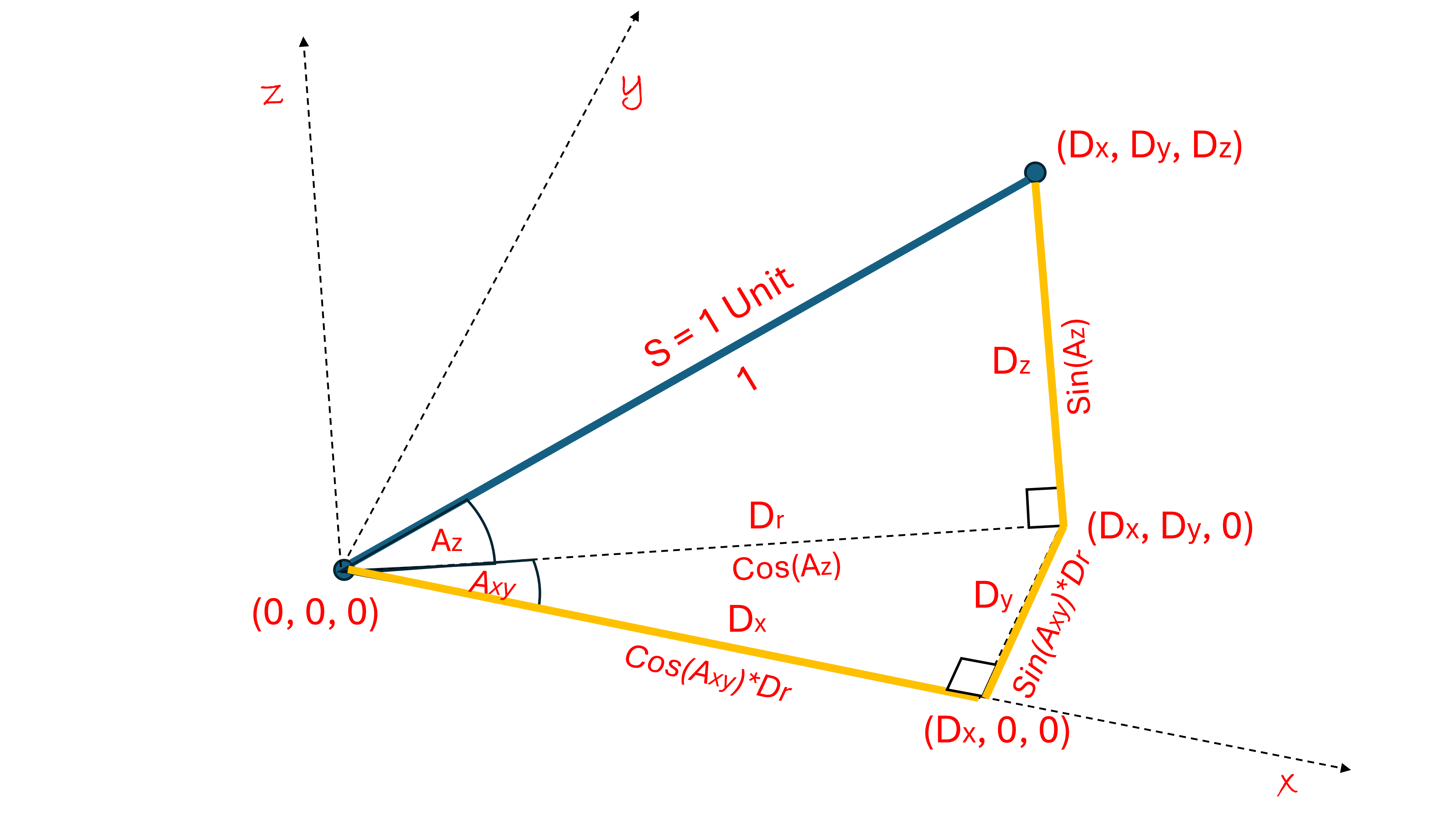
While we were drawing curves in 2-D, you might have realized that the derivative of the curve at any point (dx/dt, dy/dt), gives us the “direction” (Dx, Dy) and “speed” (S) of the point (x(t), y(t)) as it travels along the curve:
(dx/dt, dy/dt) = (Dx(t), Dy(t))*S(t)
We used the function notation to suggest that the “direction” and “speed” may also vary at every point “t” along the curve.
To illustrate this concept, let’s return to the example of a car traveling along a straight road (along the x-axis). If x(t) gives you the position of the car at any time “t”, then the distance “dx” describes the distance the car travels in short time “dt”. Thus, dx/dt gives you the velocity “vx(t)” the car is moving in the x-direction at exactly the time “t”.
dx/dt = vx(t)
Now, if I was in the car, and didn’t know exactly where I was [x(t) = ?], but I did know my speed vx(t) at every point in time “t”, then I could theoretically calculate how far I have moved by adding up all the distances “dx” that I have moved over all the short time intervals “dt”.
dx = v(t)*dt
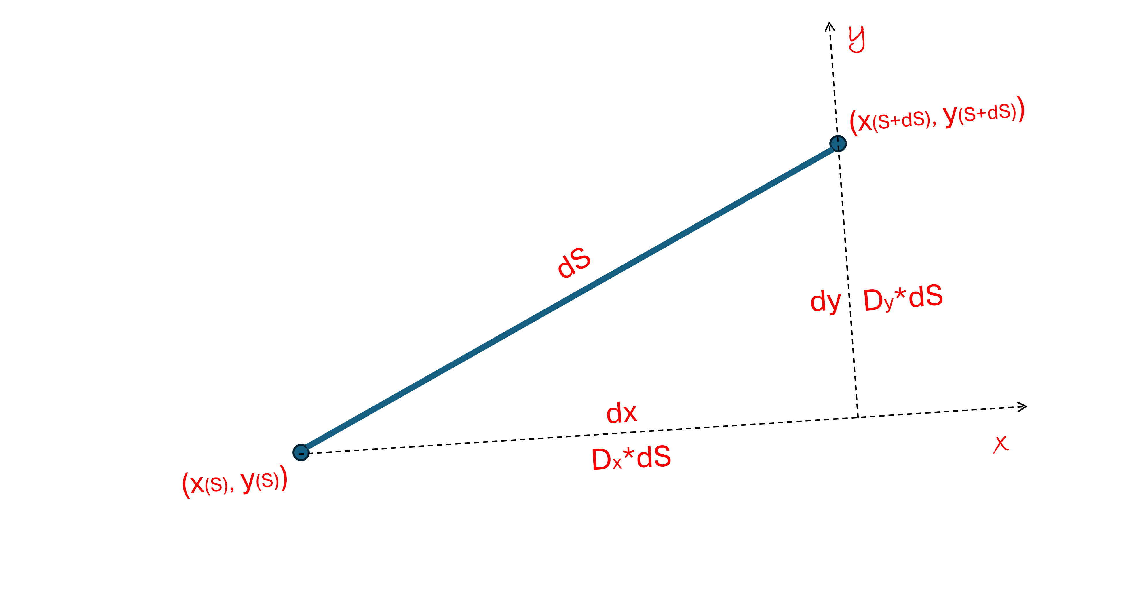
Recall that the concept of a differential, dx = x(t+dt) – x(t), involves the length and direction of an infinitesimally small segment between two points. Even though the distance between the two points gets as small as possible, we still envision that there is an infinitesimally small line segment between two points. I can figure out how far I have traveled by adding up all of these small dx segments over time.
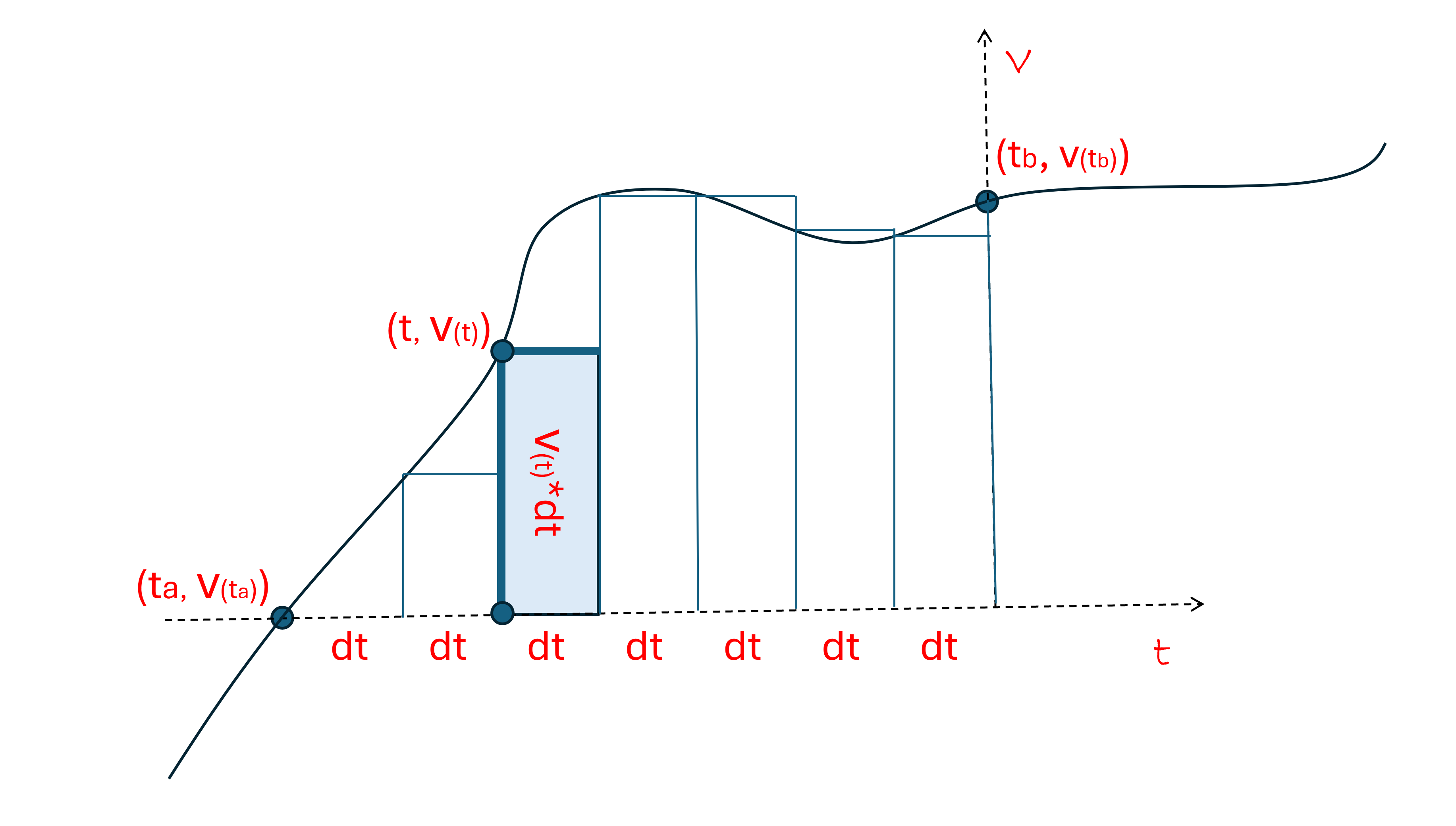
So, for instance, if I could make “dt” to be one second, and I was able to measure my starting “vx(t)” velocity at every second, I could add up the distance traveled over each of the one-second intervals and would be able to calculate the approximate distance that I moved over a certain time period. Note that this calculation would be approximate, because I could have changed velocity during any of the 1 second intervals. Please refer to the diagram below for clarity.
But remember, we make the “dt” segments infinitesimally small, and since I know the velocity “vx(t)” at every instant, I can get a much more accurate result when I shorten the time intervals. When the “dt” length approaches zero, the number of segments approaches infinity, and adding them up I should be able to calculate exactly how far I have moved from my starting point. I just have to accept the idea that I can add up an infinite number of infinitesimally small segments and still get something that makes sense.
We now look at the concept of an Integral function “I” that adds up all the infinite differential segments between a starting point “a” and ending point “b” and returns the sum of the distances between them. Since we assume that each of the “dx” segments are equal in size, we define the integral function that adds up all the differential segments between two points, x=a and x=b:
Iab[dx] = b – a (all segments “dx” are “equal” in size)
This doesn’t seem too exciting until we consider that the length of the differential “segments” might be changing in time, so that at time ta, we are at x(ta), and at time tb we are at x(tb):
Since dx = vx(t)*dt we “Integrate” both sides:
Ix(ta)x(tb)[dx] = Itatb[vx(t)*dt] so
x(tb) – x(ta) = Itatb[vx(t)*dt]
The second integral adds up all the differential elements vx(t)*dt from ta to tb (depicted by the shaded area in the diagram). At first it might seem unrealistic to solve this by adding up an infinite number of infinitesimally small segments (v(t)*dt) until a mathematician named Isacc Newton realized that the function x(t) is simply the Anti-Derivative of vx(t), and this Anti-derivative is something we might be able to determine.
So, if vx(t) = 5, then x(t) = 5*t + C (because if we take the derivative of 5*t + C we get 5), or if vx(t) = 2*t, then x(t) = t2 + C (because if we take the derivative of t2+C we get 2*t). Here we had to add on a C (meaning constant) term because when we take derivatives, all constant terms go to zero (it is easy to prove this out), so when we take Anti-Derivatives, we need to add on an unknown constant.
If we use the Anti-Derivative function “x(t) = AD[vx(t)]” then:
Since x(tb) – x(ta) = Itatb[vx(t)*dt] then
AD[vx(t)](tb) – AD[vx(t)](ta) = Itatb[vx(t)*dt]
And we have solved the integral function if we can find the Anti-Derivative “AD” of the function vx(t).
Let’s check this out, suppose:
x(t) = t2 + 5 then
v(t) = dx/dt = 2*t
This means that the velocity is 2 mph after 1 second, 4 mph after 2 seconds, 6 mph after 3 seconds, etc. It is constantly increasing. Then since AD[2*t] = t2 + C, plugging in to the Integral solution gives us:
(tb2 + C) – (ta2 + C) = Itatb[v(t)*dt]
Now since we know what x(t) is we can just plug the values directly in:
x(tb) – x(ta) = (tb2 + 5) – (ta2 – 5) and checking…
(tb2 + C) – (ta2 + C) = tb2 – ta2
(tb2 + 5) – (ta2 – 5) = tb2 – ta2
And the method checks out. It is not hard to see that this Anti-Derivative trick works wonders.
Now let’s use this to find the distance traveled along the curve from t=0 to t=1:
x(t) = t
y(t) = t2
dx/dt = 1
dy/dt = 2*t
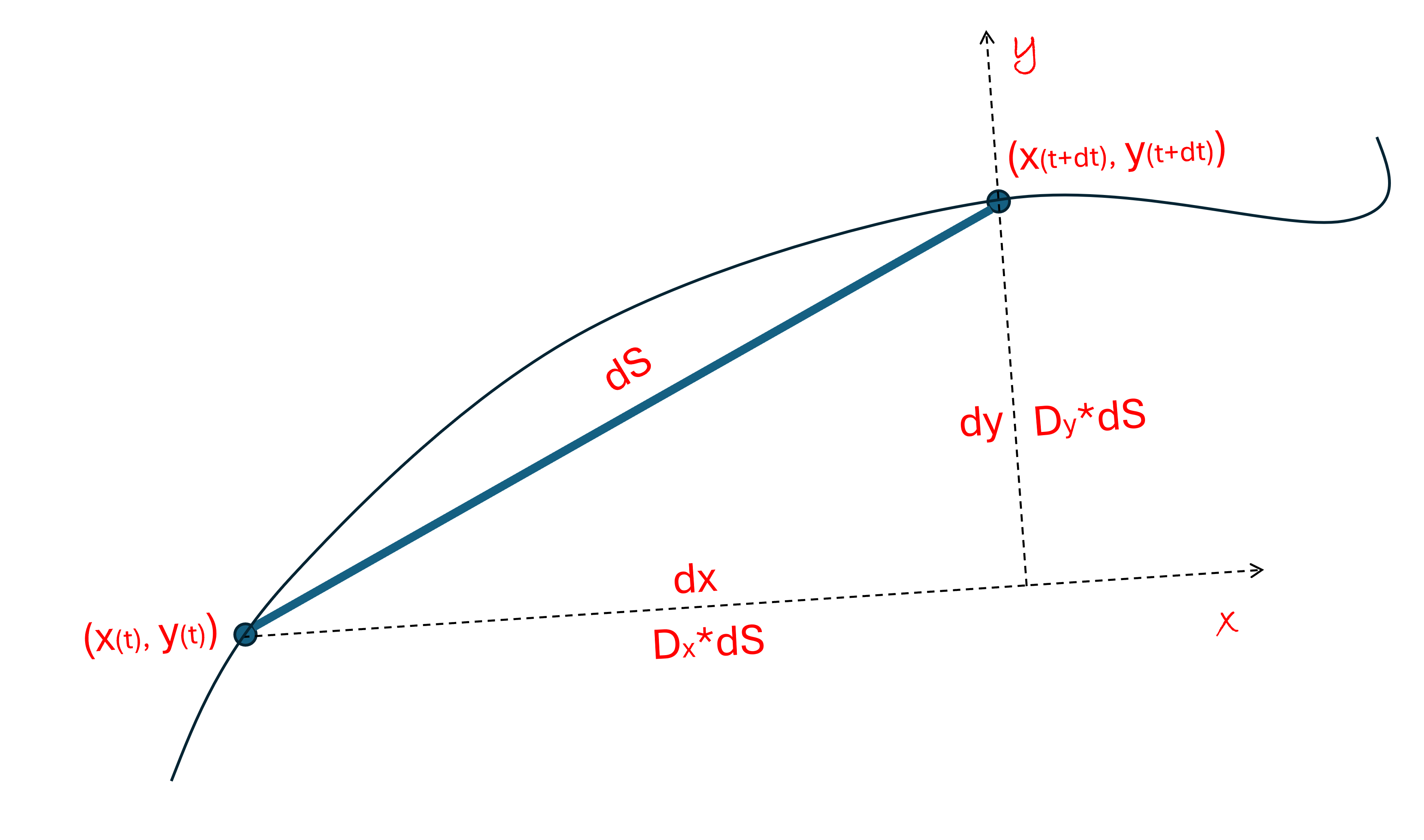
dS = (dx2 + dy2)1/2 = ((dx/dt)2 + (dy/dt)2)1/2 * dt
=(1+4*t2)1/2 * dt
Thus:
IS(0)S(1)[dS] = I01[(1+4*t2)1/2 * dt]
Looking up on integral tables:
AD[(1+4*t2)1/2]
= (1/2)*t*(4*t2+1)1/2+(1/4)*arcsinh(2*t) + C
And so, we can evaluate the Integral Equation above:
S(1)-S(0) = (1/2)*1*(4*1+1)1/2+(1/4)*arcsinh(2*1) + C
– ((1/2)*0*(4*0+1)1/2+(1/4)*arcsinh(2*0) + C)
= (1/2)*51/2 + (1/4)*arcsinh(2) – 0
= (1/2)*(2.236..) + (1/4)*(1.444)
= 1.4789…
Alright, I didn’t say that doing Anti-Derivatives are necessarily easy, but you can look most of them up on integral tables, and then you can use your calculator to plug in values at the endpoints to get the answers you are looking for.
Before you start to complain about this being too hard, Integrals are extremely useful in real world applications. Isacc Newton invented integral calculus because he was given the problem of how to hit castles with cannon balls. They knew the velocity when they fired the cannon balls, they knew the angle at which they shot the cannon ball (vx(t), vy(t)), and the downward acceleration of gravity g = -dvy/dt, and wanted to find (x(t), y(t)), the path of the cannon ball. Newton showed how they could figure it out on a scrap of paper, using a pencil and simple math (using Integrals, of course). Now you can too.