As we enter dimensions beyond our physical experience, it might help our understanding to look back and see patterns in smaller dimensions that still apply in larger dimensions. Is there such a pattern when finding directions (Dx, Dy, Dz, Dt) in 4 dimensions or larger. One obvious pattern, as dimensions increase, is the way we measure distance:
1-D: Dx2 = 1
2-D: Dx2 + Dy2 = 1
3-D: Dx2 + Dy2 + Dz2 = 1
4-D: Dx2 + Dy2 + Dz2 + Dt2 = 1
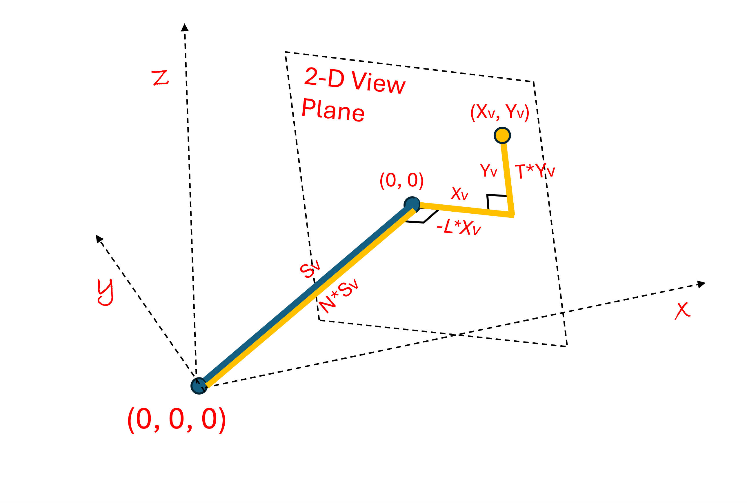
The pattern for higher dimensions is obvious. We expect this pattern to continue to any number of dimensions; we just keep adding on perpendicular triangles. See the diagram above.
There is one problem with setting directions in higher dimensions that is not so obvious. For example, in 1-D, Dx2 = 1 means that Dx = 1 or Dx = -1, this defines the directions to be along the positive or negative x-axis. So far so good. In 2-D, however, when Dy2 = 1, it forces Dx2 = 0, which does not indicate either a positive or negative direction along the x-axis. This ambiguity is due to the rotational symmetry of perpendicular lines, as we have mentioned before, you can “flip” negative and positive directions around a perpendicular direction, and nothing changes.
This ambiguity of direction exists whenever we add a new dimension. In 3-D, for example, when Dz2 = 1, it forces Dx2 + Dy2 = 0 and there are ambiguities as to where to place the direction of both the x-axis and y-axis. To a man standing exactly on the north pole, for example, every direction is south, there is no east and west. I have also heard it said that no matter how you comb the fuzz flat on a tennis ball, there will always be a part (singularity).
To deal with these ambiguities when any of our direction parameters is zero, it is helpful to fix the angles of the x-axis, y-axis, z-axis, etc. so that directions will not be ambiguous when you pass through the “singularities” where one or more of the direction parameters are forced to be zero. So a man standing on the north pole, where every direction is south, still knows which angle to face if he wants to point to Paris, France. This makes defining directions consistent.
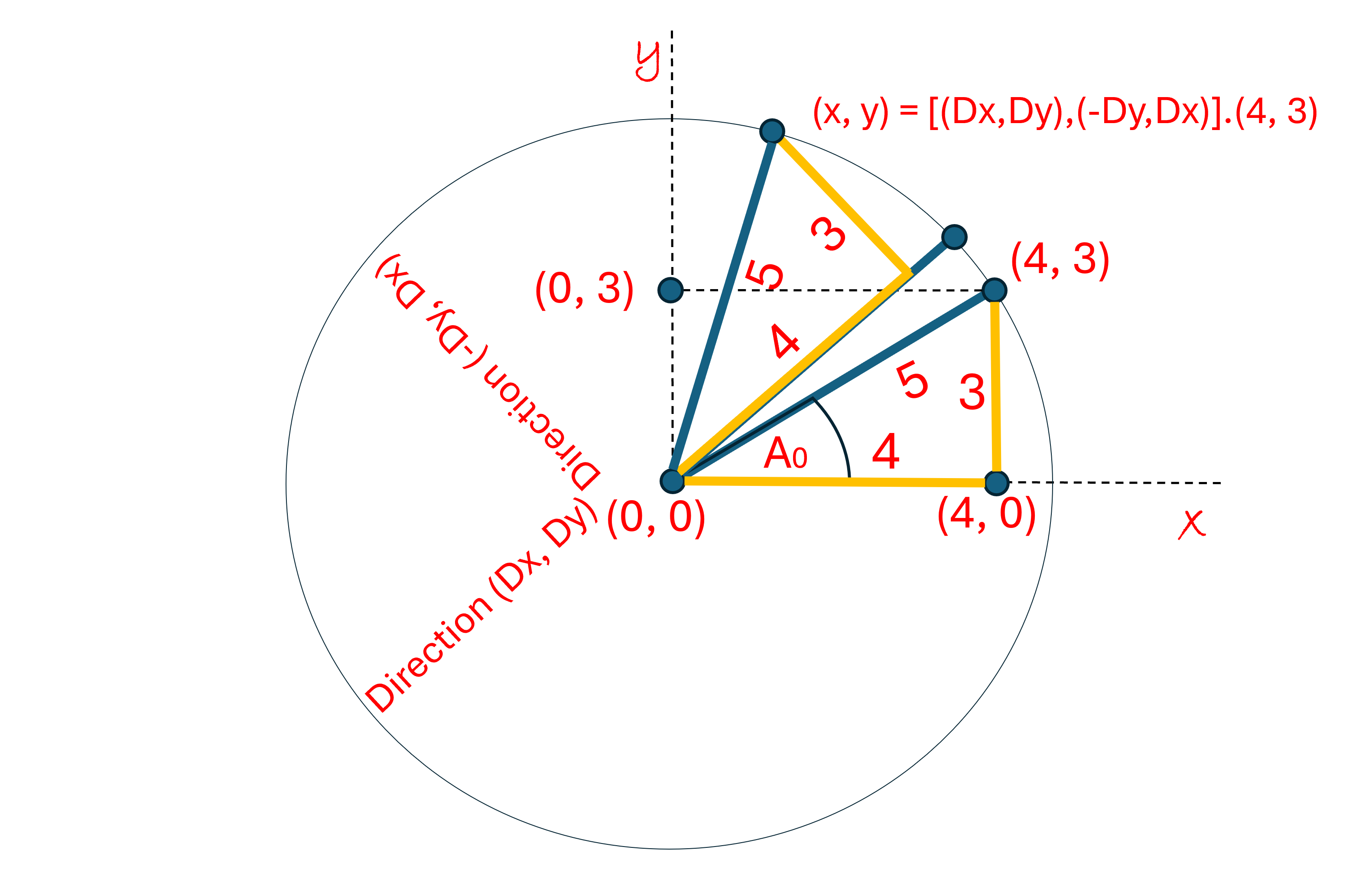
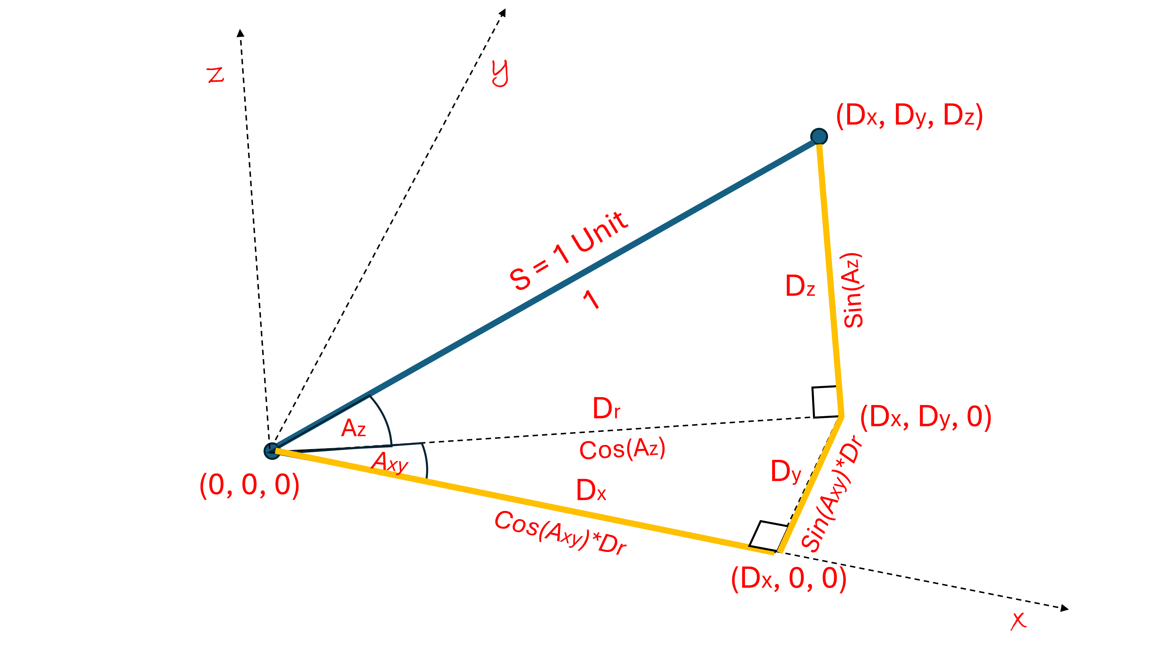
Let us look at a way to define directions as we are increasing dimensions. We defined the angle Axy to be the angle from the x-axis in the x-y plane. Then we defined the angle Az to be the angle off of the x-y plane in the z direction. Listing the direction parameters for the dimensions we know:
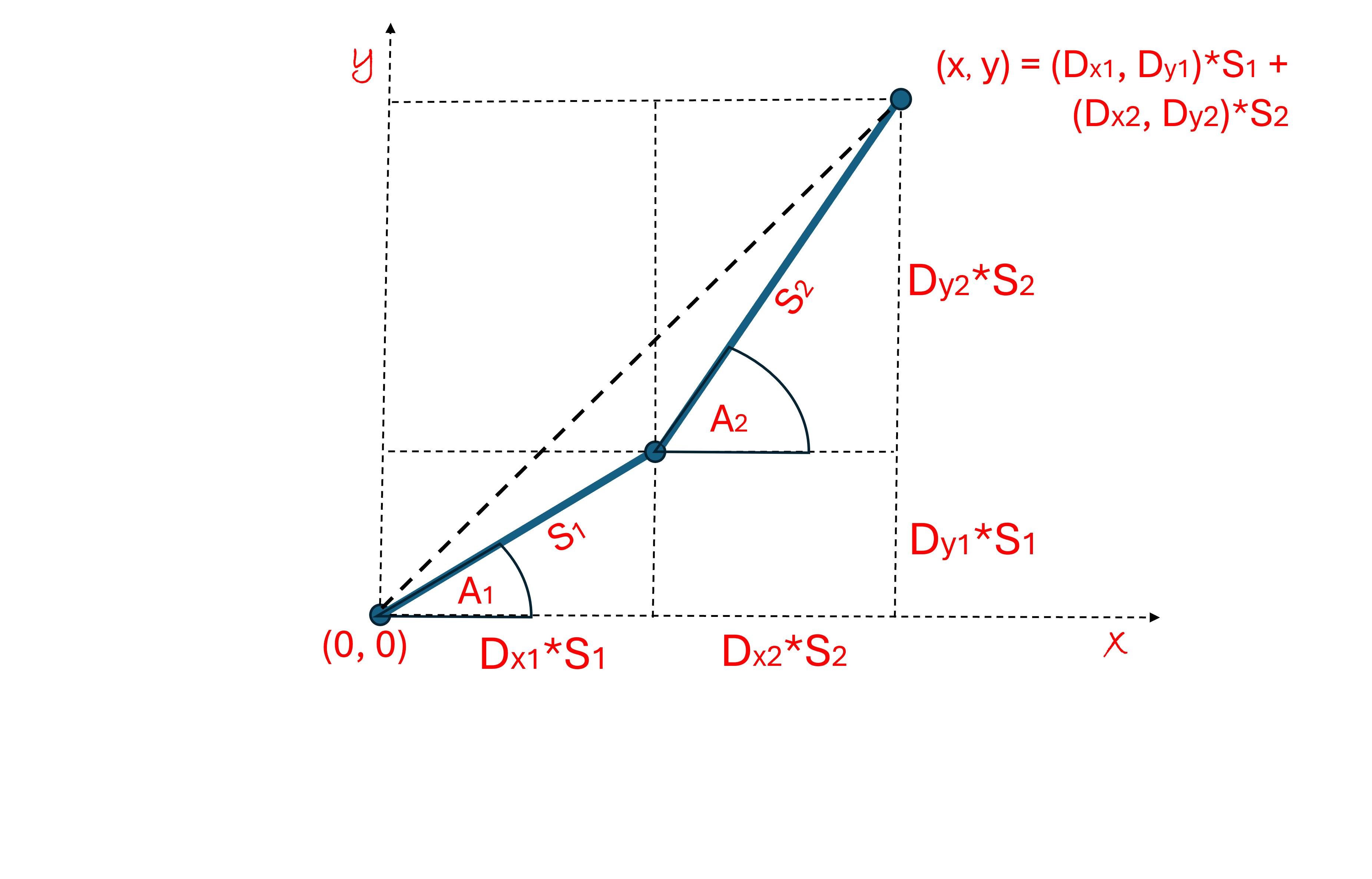
2D: D2 = (D2x, D2y) = (Cos(Axy), Sin(Axy))
3D: D3 = (D3x, D3y, D3z) = (D2x*Cos(Az), D2y*Cos(Az), Sin(Az))
= (D2x, D2y, 0)*Cos(Az) + (0, 0, 1)*Sin(Az)
We added the “2” and “3” subscripts to indicate the dimension.
It might take you a few minutes to see the pattern. Expanding into 4-D, we define the angle At to be the angle off the x-y-z space toward the t-axis, then continuing the pattern, the direction in 4-D is:
D4 = (D4x, D4y, D4z, D4t) = (D3x, D3y, D3z, 0)*Cos(At) + (0, 0, 0, 1)*Sin(At)
So putting them together and stacking them we get:
D4x = Cos(Axy)*Cos(Az)*Cos(At)
D4y = Sin(Axy)*Cos(Az)*Cos(At)
D4z = Sin(Az)*Cos(At)
D4t = Sin(At)
And we have found the Direction parameters in 4-D, and hopefully we can see the pattern that will allow us to use the same scheme to find directions in any dimension. An interesting side note: The angle in the t-direction, At, determines how close the 4-D direction is to the t-axis. When it gets close to 90 degrees, the direction is close to the t-axis and Cos(At) is close to zero, and D4x, D4y and D4z are close to zero, this restricts motion in the x-y-z space. The faster time is moving, the more restricted the motion is in 3-D space. How strange. We will see just how strange in the following post.