
Finally, we have all the tools laid out and ready, we can focus on doing something constructive, or at least interesting, with the math we have learned.
Often in architecture, engineering, physics, math, chemistry, design, artwork, or any number of creative fields, we need to build paths (lines and curves) to describe motion or outline objects.
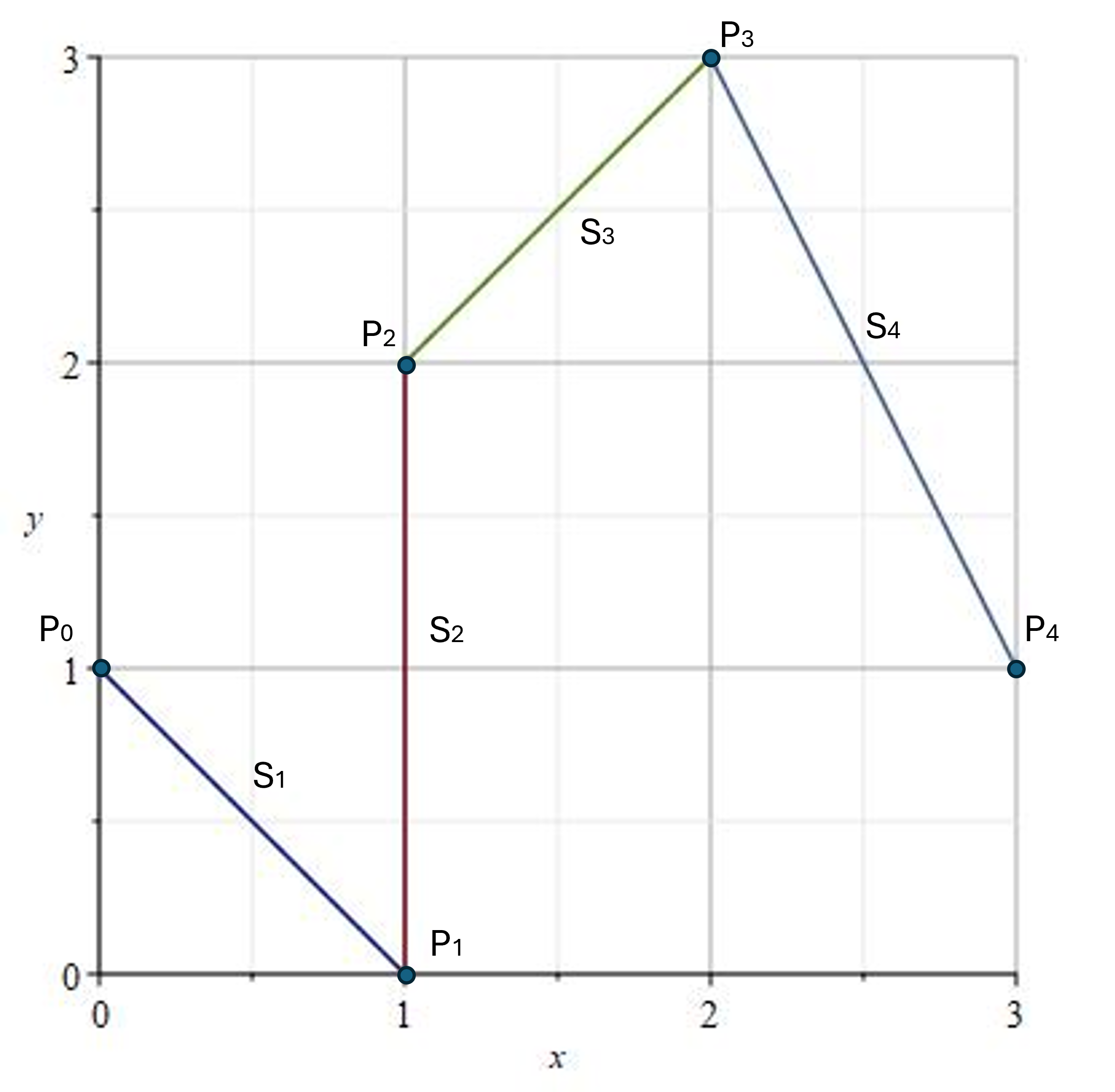
We already have drawn lines and hooked them together to make straight “angular paths”, like we did in orienteering, going in straight lines from point to point.
We start with a bunch of points placed in the order that we want our path to go through, P0, P1, P2, P3, P4, P5. We listed 5 here, but there could be any number of points on our path. We will also start by looking at just the “x” coordinate of the first segment between the first two points, P0 and P1. As we have seen, we can expand this into more dimensions (x, y, z) later.
Let’s look at the, now familiar, equation for the x coordinate of a line between the first two points P0:(x0, y0) and P1:(x1, y1):
x(S) = x0 + Dx0*S
The independent variable “S” marks the distance traveled along this segment from P0, and the Dx0 is the x-direction of this segment between P0 and P1. “S” starts at S=0 (at P0) and goes to S=S1 (at P1), where “S1“ is the distance of the line segment between P0 and P1.
Since this first segment of the path stops when the line reaches the end point (x1, y1) after traveling the distance between them, S1:
x1 = x(S1) = x0 + Dx0*S1
thus
x1 – x0 = Dx0*S1 and
Dx0 = (x1 – x0)/S1
Substituting this expression for Dx0 into the equation of the line we get:
x(S) = x0 + (x1 – x0)*S/S1
Notice that the ratio S/S1 can be thought of as a percentage and ranges from 0 to 1 as S goes from 0 to S1. To avoid calculating lengths of the segments, we can use the substitution:
t = S/S1
into the equation for a line and we get:
x(t) = x0 + (x1 – x0)*t where t goes from 0 to 1.
This turns out to be a very convenient way to write the equation of a line between two points. With this equation, x(0) = x0 and x(1) = x1, and “t” marks the “percentage” traveled along the line segment, from 0% (t=0) to 100% (t=1).
Expanding this into two dimensions we get the equations for all 5 segments between the 6 points:
Segment 1: (x(t), y(t)) = (x0, y0) + (x1-x0, y1-y0)*t
Segment 2: (x(t), y(t)) = (x1, y1) + (x2-x1, y2-y1)*t
Segment 3: (x(t), y(t)) = (x2, y2) + (x3-x2, y3-y2)*t
Segment 4: (x(t), y(t)) = (x3, y3) + (x4-x3, y4-y3)*t
In each case, “t” goes from 0 to 1. This is written out in full detail to make sure that you can see the pattern. In two dimensions you can find the length of Segment 1 by S12 = (x1-x0)2 + (y1-y0)2. The others are not written out, the pattern should be obvious.
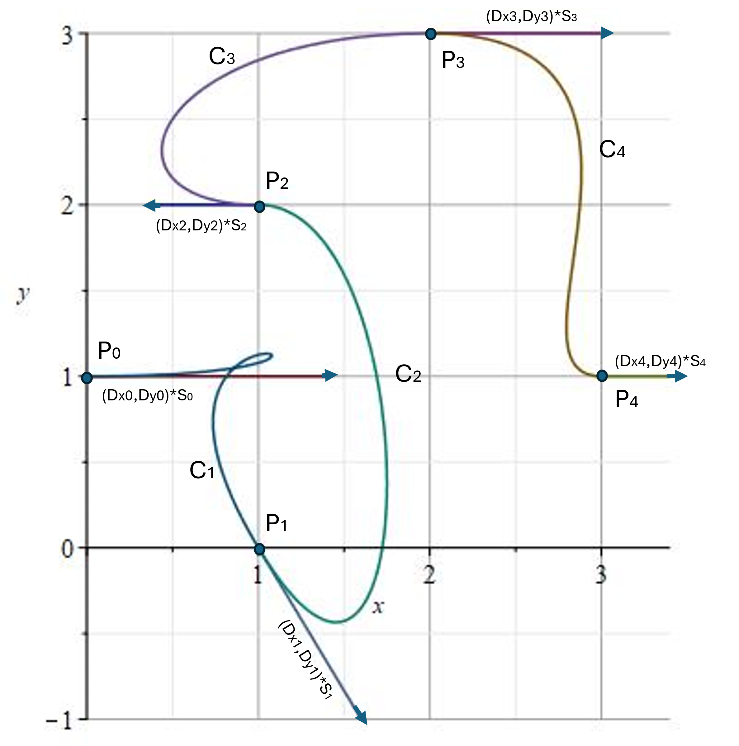
Alright, we can draw lines between the points. Now let’s look at drawing curves between the points. This becomes a bit harder to pin down because there literally are an infinite number of curves that could be drawn between these same 5 points. We will have to specify the kind of curves we want.
We will learn how to draw curve segments between the points and put them together smoothly to form any continuous path we desire. We could even use this math to find an equation that describes the path of a fly walking around on the ceiling.
One common way of doing this is to use a method called “cubic splines”. With this method the coordinates of each curve are written as a “cubic” equation in t:
x(t) = c0 + c1*t + c2*t2 + c3*t3
where we can pick any numbers we want for c0, c1, c2, and c3. The numbers we pick determine the shape and position of the curve. We can also write this expression using the “dot” product we have discussed before:
x(t) = (c0, c1, c2, c3).(1, t, t2, t3)
The “c”s are called the coefficients and the powers of “t” are called the basis functions. We can now take the derivative of the x-coordinate as we learned in the last post.
dx/dt = (c0, c1, c2, c3).(0, 1, 2*t, 3*t2)
as you recall, we can use these derivatives to find the direction of the tangent line at any point “t” along the curve. As it turns out, we now have all the tools necessary to draw a “cubic spline” curve between the points.
We can pick “t” to be a “percentage of the curve” where “t” starts at t=0, the beginning of the curve, and goes to t=1 at the end of the curve (similar to how we drew lines). And so:
x(0) = (c0, c1, c2, c3).(1, 0, 0, 0) = x0 (Substitute t=0 into the equations above)
x(1) = (c0, c1, c2, c3).(1, 1, 1, 1) = x1 (Substitute t=1 into the equations above)
written out this means:
c0 + 0 + 0 + 0 = x0 and
c0 + c1 + c2 + c3 = x1
and we have found that the coefficient c0 = x0 (the x-coordinate of the starting point) and the sum of the coefficients must add to x1 (the x-coordinate of the ending point). This meets the conditions that the curve will start at the beginning point and end at the ending point. We still need some more conditions to determine what the other c’s will be.
It is natural to also place conditions on the direction that the curve leaves the starting point and the direction it arrives at the ending point. This is determined by the tangent direction (derivatives) at these points:
dx/dt(0) = (c0, c1, c2, c3).(0, 1, 0, 0) = S0*Dx0
dx/dt(1) = (c0, c1, c2, c3).(0, 1, 2, 3) = S1*Dx1
We can set S0, S1 and the directions Dx0 and Dx1 to be whatever we want and we can immediately see:
c1 = S1*Dx0
c1 + 2*c2 + 3*c3 = S2*Dx1
We have determined c0 and c1 from the starting point and the direction of the tangent at that point. We can use substitutions to find the rest. We have 4 equations and 4 unknowns and so we do this:
3*c0 + 3*c1 + 3*c2 + 3*c3 = 3*x1 (multiply the sum by 3)
c1 + 2*c2 + 3*c3 = S1*Dx1 (from above)
Subtracting the second equation from the first and making substitutions for c0 and c1:
3*c0 + 2*c1 + 1*c2 + 0*c3 = 3*x1 – S1*Dx1 (making subs)
3*x0 + 2*S1*Dx0 + c2 = 3*x1 – S1*Dx1 (solve for c2)
c2 = 3*x1 – 3*x0 – S1*Dx1 – 2*S0*Dx0 or
c2 = 3*(x1 – x0) – (S1*Dx1+2* S0*Dx0)
c3 = x1 – (c0 + c1 + c2) (rearranging the sum)
c3 = x1 – [x0 + S0*Dx0 + 3*(x1 – x0) – (S1*Dx1 + 2*S0*Dx0)]
c3 = -2*(x1 – x0) + S1*Dx1 + S0*Dx0
and now we have found all the “c” coefficients.
We can now draw the curves between the points if we know the starting point (x0, y0), the ending point (x1, y1), the starting direction (Dx0,Dy0) and the ending direction (Dx1, Dy1). The S0 and S1 variables are arbitrary and can be varied to taste. We now plug all of these coefficients into our original curve:
x(t) = (c0, c1, c2, c3).(1, t, t2, t3)
dx/dt = (c0, c1, c2, c3).(0, 1, 2*t, 3*t2) = S0*Dx0 (tangent direction)
the y(t) equation follows exactly the same pattern (just substitute “y” for “x” in all the equations). Voila, we have found a “cubic” curve that passes through these points and has these tangent directions.
We can now do the same for all of the curves between each pair of points, drawing curves through all of the points. There is a little bit of wiggle room in these curve equations. The S0, S1, … and direction parameters for the tangents at the points can be set at will. Since the direction vectors are the same at the points, the curve will smoothly pass through the points in the same direction. These direction vectors show the “nose” direction (Dx,Dy) and “speed” (S) that a fly would be traveling if it were walking along the curve. It is fun to program these equations into a computer that draws them and watch the curves change as you change the location of the points and the directions and magnitudes of the tangents at the points. This is how most modern, curve-fitting software works.
Of course, you can use another set of “basis functions” rather than just the powers of “t”, if you wish, to possibly get a better fit on your curves. You might also want to impose other conditions, such as minimum curvature. Just remember, if you use more basis functions, you will have more equations to solve for, you will need more conditions, and you might need some experience in “linear algebra” to solve for the coefficients. Happy curving!

