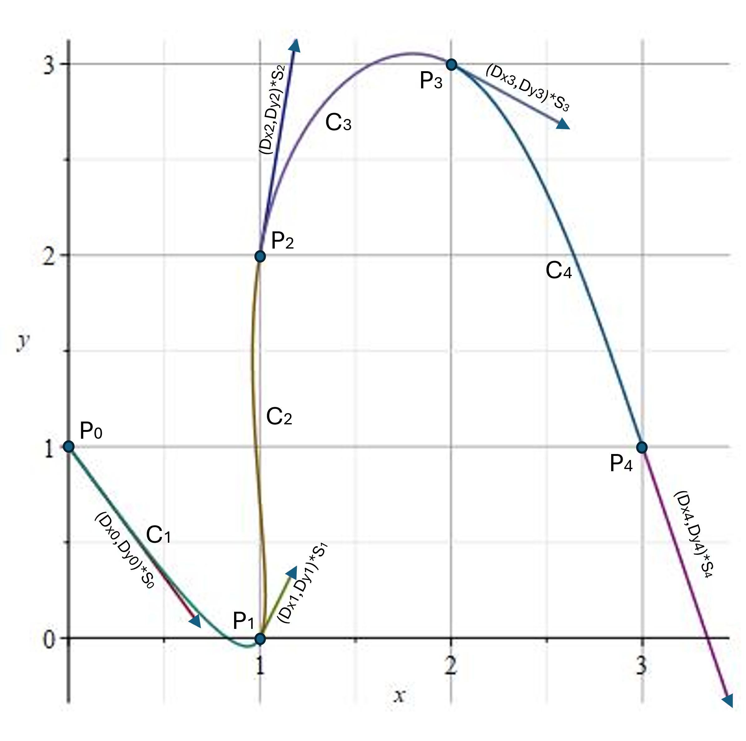
Alright, let’s start with a problem that you might want to solve if you were driving a “space shuttle” in the middle of deep space (perhaps in a video game). You have 5 orbs floating in space at the same locations of the 5 points picked in the “Building a Curved Path” (cubic splines) post a few weeks ago.

The problem is: You want to fly through the same 5 points and catch the orbs in your net as you pass by them.  You want to minimize the fuel that it takes to “accelerate” your shuttle along a curved path passing through the 5 points.  What would be your optimum path?

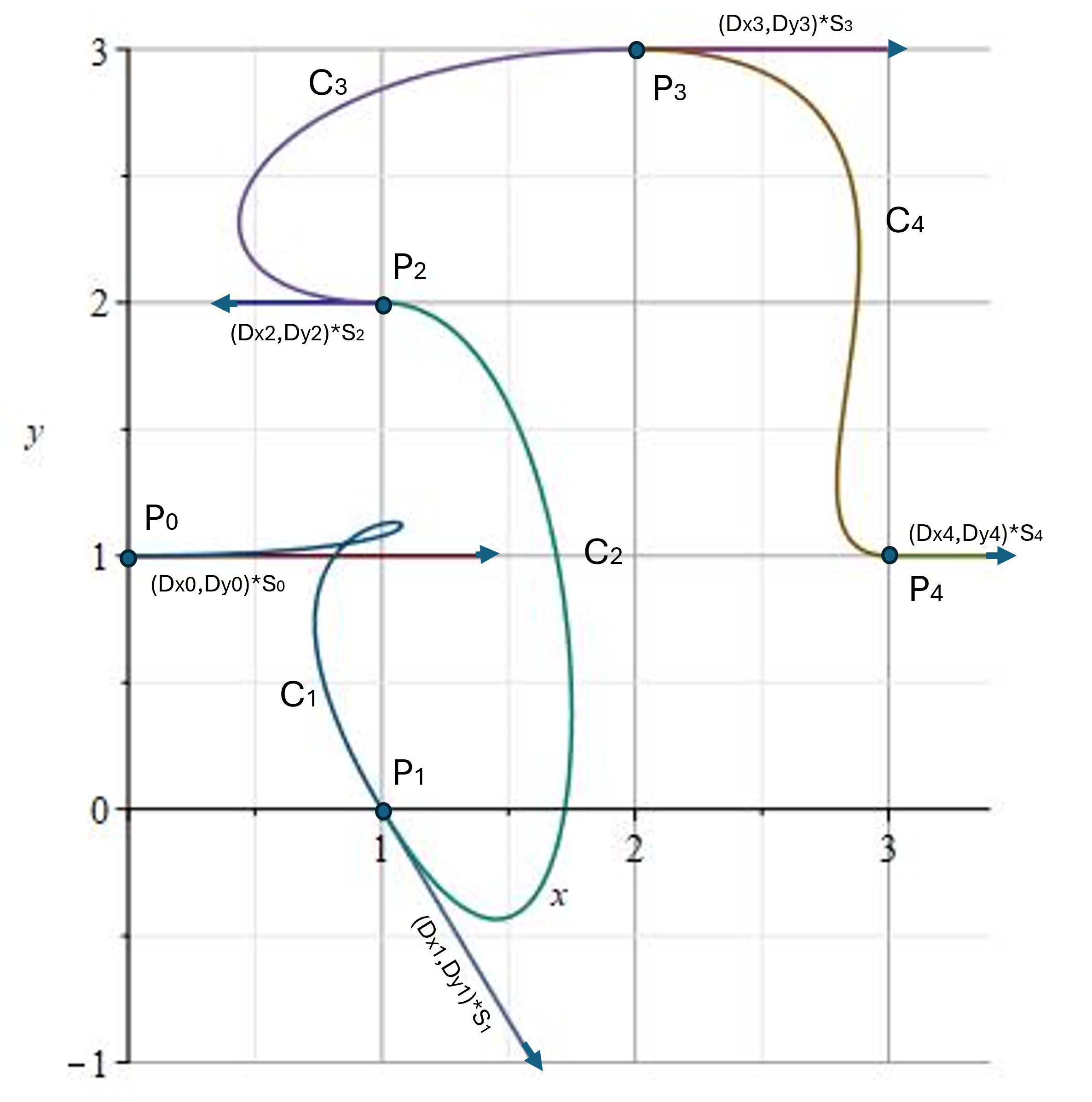
You can set the speed and direction you will be traveling as you fly by each of the points.  It is obvious that the speed and directions we picked in the original “Curved Path” would not give you the optimal path, it even makes a “curlycue” loop.  So how would you figure out the optimal speeds and directions that will give you an optimal curve for the shuttle?

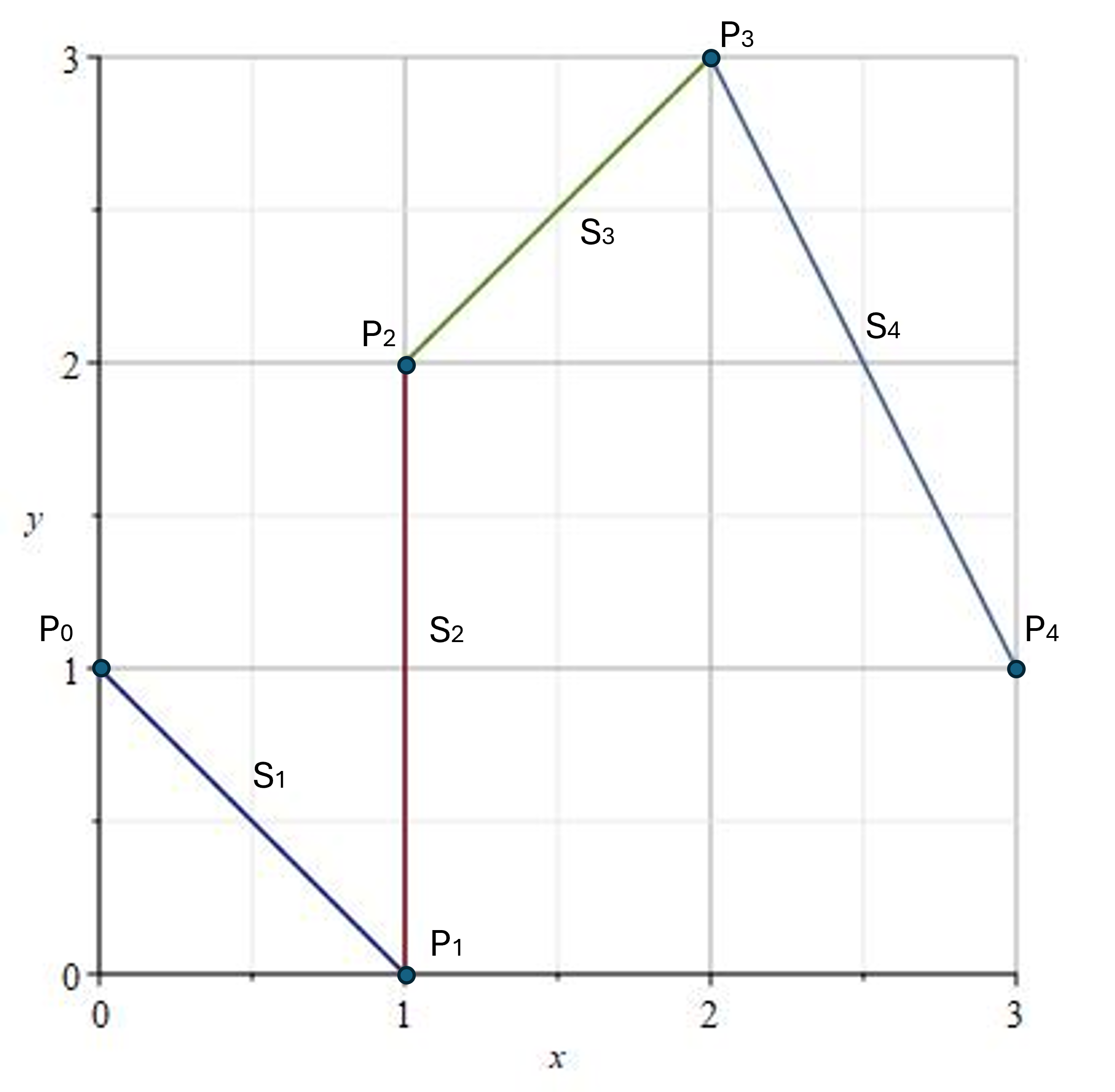
One way is to follow a straight line between points, stopping at each point, then turning toward the next point and speeding up again. You would have to speed up, then slow to a stop and pick up an orb at each point.  To conserve fuel, you would not be able to speed up very fast between points and would end up slowly “coasting” along the lines between each of the points and you must use your fuel to stop again.  This would work, but it might be slow and boring, especially if the points are spread far apart.

The way that would be most fun is to build up some speed and figure out the optimal way to change direction so that your net will scoop up the orbs on the fly as you pass by them.  Keep in mind that every time you change direction, or accelerate, you are using fuel.  Coasting in a straight line, with zero acceleration, does not cost you any fuel.

So, the idea is to minimize your acceleration along your whole path (x(t), y(t)).  Recall that your direction and speed (velocity “v”) is determined by the derivatives of your position along the path:

  (v_x(t), v_y(t)) = (dx/dt, dy/dt)

Your acceleration “a” is determined by how fast your velocity is changing.  And so, the derivative of your velocity is your acceleration:

(a_x(t), a_y(t)) = (dv_x/dt, dv_y/dt).

Now comes the key innovation: to save time and typing, we are going to start using the notation of “linear algebra” to solve the problem.  We will use bold-faced letters (p, v, a) (position, velocity, acceleration) to denote these “vector” entities, with the understanding that these bolded letters represent the whole “vector” consisting of all the components:

p(t) = (x(t), y(t))
v(t) = (v_x, v_y)
a(t) = (a_x, a_y)

Now we take this a step further, we will use the same “cubic” basis we used in “Building a Curved Path” to write out the curve, we will express this as the vector “b”:

b(t) = (1, t, t², t³)

and using the “dot product” notation we write the equations:

x(t) = (c_x1, c_x2, c_x3, c_x4)^.(1, t, t², t³) = c_x^.b(t)
y(t) = (c_y1, c_y2, c_y3, c_y4)^.(1, t, t², t³) = c_y^.b(t)

where the “c_x, and c_y” vectors of coefficients that determine the shape of the curve. Please refer back to the “Building a Curved Path” post for clarity.  So, the shortened notation for the equations of the curve is:

p(t) = (x(t), y(t)) = (c_x^.b(t), c_y^.b(t)) = [c_x, c_y]^.b(t)

There is conserved complexity in this simplified notation.  First of all, the [c_x, c_y] is a vector of vectors, representing both the 4 coefficients for the x(t) (c_x) and the 4 coefficients for the y(t) (c_y) functions. (8 coefficients in all).  Now you can see why we save a lot of typing with this notation.

[c_x, c_y] (a vector of vectors) is also referred to as a “matrix” the 4 c_x coefficients are sometimes written as the first row and the 4 c_y coefficients as the second row, so this “matrix” is referred to as a 2×4 matrix (C).  And again, by conservation of complexity, we can also write matrixes as bold capital letters:

C =  [c_x, c_y]

Thus, the equation for the curve can be written in matrix form simply as:

p(t) = [c_x, c_y]^.b(t) = C^.b(t)

and we just need to find the 8 coefficients in the C matrix to completely determine the curve.

C is a 2×4 matrix and b(t) is a 4×1 vector.  This notation not only makes things easier to write down, but it turns out to be very helpful (similar to the reason we used the “dot product” notation).

Another reason this is so helpful, is because if you want to take derivatives you just need to find the derivatives of b(t), which is more simple than taking derivatives of x(t) or y(t):

b(t) = (1, t, t², t³)
db/dt = (0, 1, 2*t, 3*t²)
d²b/dt² = (0, 0, 2, 6*t)

The expression d²b/dt² means the “second derivative” of b, or the derivative of the derivative.

So, since the C matrix does not change when you take derivatives only on the b(t) vector,

p(t) = (x(t), y(t)) = C^.b(t)
v(t) = (v_x, v_y) = C^.(db/dt)(t)
a(t) = (a_x, a_y) = C^.(d²b/dt²)(t)

and we have found the linear-algebra equations for three important characteristics of this curve, the position, velocity, and acceleration at every point “t” along the curve.

Note that we have not changed the equations, just how we write them down. Believe it or not, this notation makes it much easier to find the unknown coefficients in the matrix C that defines the curve.  First we must specify where we want the curve to go.

Again, we set the condition that when t=0, the curve starts at the point (x₀, y₀).  we also set the velocity at t=0 to be (v_x0, v_y0).  Now we then have these 4 known numbers, we need 8 unknown numbers (in the matrix C).  From the principles of “linear algebra” if we have 8 known numbers, we can find the 8 unknown numbers in C. We still need 4 more known numbers.

We can now set the ending point to be (x₁, y₁) and the velocity to be (v_x1, v_y1) when t =1.  These are the 4 more conditions (known numbers) that we need.  These conditions at the “endpoints” are called the boundary conditions.  If we have 8 boundary conditions, then we generally can solve for the 8 unknown coefficients.

Here is how: First, write down the equations for the boundary conditions:

p(0) = (x(0), y(0)) = (x₀, y₀) = C^.b(0)
p(1) = (x(1), y(1)) = (x₁, y₁) =  C^.b(1)
v(0) = (v_x0, v_y0) = C^.(db/dt)(0)
v(1) = (v_x1, v_y1) = C^.(db/dt)(1)

Then write these boundary points (Bp) in matrix form:

Bp = [(x₀, y₀), (x₁, y₁), (v_x0, v_y0), (v_x1, v_y1)]
=  C^.[b(0), b(1),  db/dt(0),  db/dt(1)]    (substitute for t)
= C^.[(1,0,0,0), (1,1,1,1), (0,1,0,0), (0,1,2,3)]
= C^.B (where B is the matrix […] above)

So these boundary conditions boil down to an equation of matrixes:

Bp =  C^.B

We know Bp, it is a 2×4 matrix of boundary points and velocities.  We know B, it is a 4×4 matrix of basis functions and their derivatives at the boundary endpoints (t=0, t=1).  We just need to find the C matrix (2×4).  It wouldn’t it be nice if we could somehow “divide” by B so we can determine what the C matrix is.

It turns out that linear algebra gives us a way to do this by finding the inverse matrix of B, called B^-1.  Inverse matrixes can be found on many calculators and computers. If you “dot” a matrix by its own inverse you get the “identity” matrix Id (we discussed earlier).  Dotting anything with the identity matrix is just like multiplying by number 1, anything dotted with the identity matrix just returns itself:

B^.B^-1 = Id = [(1,0,0,0), (0,1,0,0), (0,0,1,0), (0,0,0,1)]

In this case the calculator shows (check it out):

When
B = [(1,0,0,0), (1,1,1,1), (0,1,0,0), (0,1,2,3)]
then
B^-1 = [(1,0,-3,2), (0,0,3,-2), (0,1,-2,1), (0,0,-1,1)]

And

C^.Id = C

So dotting the above equation (Bp =  C^.B with B^-1) on both sides gives you the C matrix:

Bp^.B^-1 = C^.B^.B^-1 = C^.Id = C

We have found C, so now we can now write the equation for the curve:

(x(t), y(t)) = C^.b(t)
= (Bp^.B^-1)^.b(t)
= Bp^.(B^-1.b(t))
= Bp^.g(t)

And yet again we have defined a new vector:

g(t) = B^-1.b(t)

called a “Green’s Function”.  Once we have this Green’s Function g(t), we just “dot” it with the Boundary matrix Bp and get the curve that fits these boundary conditions.  Let that soak in for a while.  All you have to do is change the Boundary conditions matrix Bp (the beginning and ending points and velocities) dot it with g(t) and you will automatically get the equations for the curve that “magically” matches these boundary conditions (at t=0 and t=1).  All of the “hard work” needed to find the C coefficients is contained in the Green’s function.  This makes drawing and hooking together the curves easy, if we know what the points and velocities are at the endpoints of the curve.  Let’s list out the Green’s function:

g(t) = (1-3*t²+2*t³, 3*t²-2*t³, t-2*t²+t³, -t²+t³)

This same Green’s Function works for all dimensions. It is easy to see how to extend this to 3-Dimensions, just put the “z” boundary conditions into the Bp matrix and it solves for z(t).

Up to this point, in solving our problem, we have made some great progress with linear algebra notation, but we still have not found the optimal velocities (speed and direction) through the points that will minimize the acceleration along the path.  However, I think that this is enough for now.  Let’s take a breather.  It might take a while for the “linear algebra” notation we have learned to make sense.

I encourage you to write out the matrixes and see specifically how these dot products work. We will continue to solve the optimal curve in our next post.